Designing Fast BI Reports

Overview

When creating BI reports, performance can become an issue – especially if you are new to CMiC Analytics. As a user, you might expect that any report you create in CMiC should load quickly and show all the data you need in one tabular view. However, this is not the case with an application like CMiC Analytics, where users can easily run into performance issues due to poor report design.

When designing for performance, it is useful to think more like a developer. Developers increase the performance of programs by limiting the information that is displayed to only what is needed in any given moment. They do this by creating views with built-in filters, a limited amount of columns, or by requiring the user to specify filters. They may also take more technical approaches to optimize the speed of a query by doing fewer calculations, for example. Finally, developers make use of “context variables” which exist in some views.

Below you’ll find some approaches to troubleshoot and improve the performance of BI reports.

• Designing Fast BI Reports
• • Overview
  • Troubleshooting
  • • Timeout Errors
    • BI Performance Analysis Report (Patch 17)
    • Re-creating the Visualization
    • • Re-creating Backwards
      • Re-creating Forwards
      • One Visualization for Each Folder
  • Filtering Data
  • • Context Variables
    • Catalog Builder Filter
    • Query By Example
    • Page Filters and Substitution Variables Without the Use of Joins
    • Page Filters with the Use of Joins
    • Table Pivot Filters
  • Minimizing Joins
  • • Building Better Joins
  • Calculated Fields
  • Slow Views

Troubleshooting

Timeout Errors

If you’re experiencing timeout errors, you will not be able to follow the troubleshooting steps in this article without creating another BI report from scratch (see section on re-creating the visualization). However, if you understand the cause of the timeout, you can disable the Autoload Data option to prevent the BI report from loading. Then, you can make changes to the dashboard that improve the performance before enabling the Autoload Data option again.

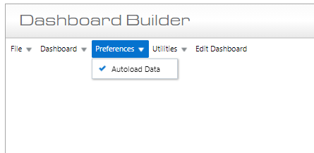
Note that the Autoload Data option is a user setting and not an attribute of the dashboard. Therefore, it can be enabled/disabled when Dashboard/Query Builder is opened - before a BI report is opened.

BI Performance Analysis Report (Patch 17)

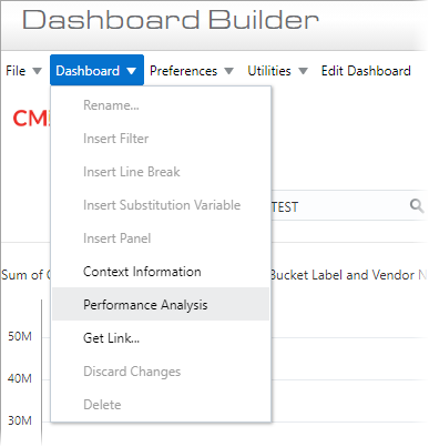
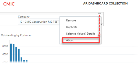
A good starting point for understanding the performance of a BI report is to run the Performance Analysis option from the Dashboard/Query menu.

The pop-up window displays the load time, folder usage, and aggregations present in each visual on a dashboard or query.

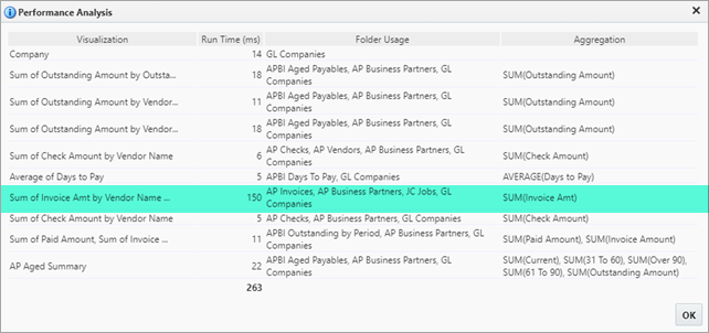
From this information, you can determine where to focus your efforts – in the above example, one visualization stands out with a 150 millisecond load time. It is almost 10 times slower than the rest of the visualizations. You can see that it uses the following folders: AP Invoices, AP Business Partners, JC Jobs, and GL Companies. It also has an aggregation: SUM(Invoice Amt).

There are some possibilities as to why this visualization is taking the longest to load. Perhaps it is aggregating more data points than the others. Maybe it lacks a filter unlike the other visualizations. Aggregating data from every invoice on every job (no matter the status) may be excessive, unless you want that. It is also possible that the underlying database table/view is not optimal and a faster alternative exists in the data catalog.

Re-creating the Visualization

Once the most problematic visualizations are identified, it is important to dig deeper to understand what exactly is slowing down the load time. With experience, you may be able to determine the reason just by examining the visualization, folders being used, and calculated fields. However, the most reliable way to troubleshoot the issue is to re-create the visualization step by step.

You may find that a performance issue is caused by a single field in a visualization. This is likely when a calculated field is used. It may also be caused by a join between two folders (selected fields from two different folders).

Re-creating Backwards

This is a procedure that has been developed by CMiC support to isolate the cause of a slow report:

1. Create a duplicate of the visualization.

2. Remove a single field from the visualization. This may be a column in a table, a series in a bar chart, etc.

3. Observe the difference in load time.

4. Repeat the above 3 steps until no fields are left in the visualization.

During this process, you may notice that the load time is dramatically different when a particular field is removed.

Re-creating Forwards

Sometimes working backwards is inconvenient, especially when the visualization is so slow that it slows down the whole troubleshooting process. In those cases, another procedure can be followed:

1. Create an empty visualization.

2. Select all the folders and fields required in the original slow visualization.

3. Apply the same filters as shown in the original slow visualization.

4. Drag a single field into the visualization. This may be a column in a table, a series in a bar chart, etc.

5. Observe the difference in load time.

6. Repeat Step 4 and Step 5 until you have re-created the original visualization.

During this process, you may notice that the load time is dramatically different when a particular field is added.

One Visualization for Each Folder

The above procedures (re-creating the visualization forwards and backwards) may not give a clear reason for the slow load time. Therefore, it may be useful to look at the load time of individual folders in the visualization. It can help you find out whether one folder is noticeably slower to load than the other folders, or whether a folder join is causing the issue. The procedure is:

1. Create an empty visualization.

2. Select a single folder with the fields that are selected in the original visualization.

3. Apply a filter to the visualization (if one is applied on the original visualization).

4. Drag a single field in the visualization. This may be a column in a table, a series in a bar chart, etc.

5. Observe the difference in load time.

6. Repeat Steps 4 and 5 until all of the required fields have been added.

7. Repeat Steps 1-6 separately for each folder selected in the original visualization.

Often, this troubleshooting procedure shows how folder joins affect performance, as well as how filtering affects different folders. In some cases resolved by CMiC Support, it was determined that data duplication from poorly selected joins was the cause of the performance issue.

Filtering Data

One of the most common reasons for poor performance in BI reports is the lack of data filtering. A report that contains Job Cost Transactions, for example, could have thousands or hundreds of thousands of data points across all jobs. This would not load very quickly in a BI report. Therefore, it is highly recommended to set up some kind of required filter on every BI report.

Some filtering methods are better than others. Below, you will find each method ranked in order of decreasing performance. Each method is described in further detail in the following sections.

1. Context Variables

2. Catalog Builder Filter

3. Query By Example

4. Page Filters and Substitution Variables Without the Use of Joins

5. Page Filters with the Use of Joins

6. Table Pivot Filters

Making a page filter or substitution variable required involves using the Value Required feature in each visualization setting. This feature prevents the visualization from loading until a value is selected. More information about each of these methods is available in the Catalog Builder and Dashboard Builder reference guides.

Context Variables

Using context variables is the ideal method to filter data in CMiC. However, it is only possible to use them on a select group of folders.

Context variables are special, pre-defined filters that developers define for specific database views. These context variables can be used in BI by referencing them in filters or substitution variables. For example, the GL Accounts folder accepts a context variable called ACC_CODE. On a page filter designed to filter on the Account Codes, the Context Variable property in the page filter settings should be set to ACC_CODE.

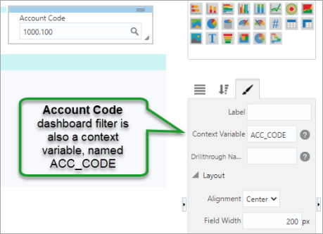
When a value is specified in that page filter, the system assigns a value to ACC_CODE, which gets used to filter the GL Accounts folder before it is loaded. This is the reason context variables perform so well.

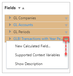
To check what context variables are supported by a folder, click the down arrow next to the folder in the selected fields section on the right of the screen.

Note that page filters and substitution variables, even without context variables, are still valuable ways to filter data. They are described in further detail in the sections below.

Catalog Builder Filter

Filtering data in Catalog Builder can be done by selecting the [Edit Filter] button when a folder is selected. You can use Oracle SQL code to specify a filter. Note that this filter gets applied to every BI report where the folder is used. Therefore, it may or may not be a good option for your use case.

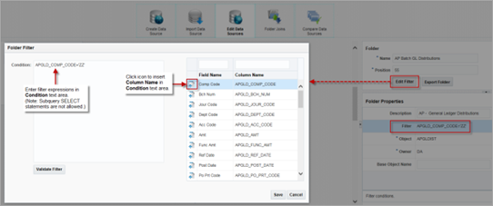
If you find that you’ll use this folder a lot with a specific filter, you can make a copy of it and apply a filter to it. For example, you can create a copy of the “AP Batch GL Distributions” folder shown above and name it “AP Batch GL Distributions VERSION 2” and apply a filter to it.

Query By Example

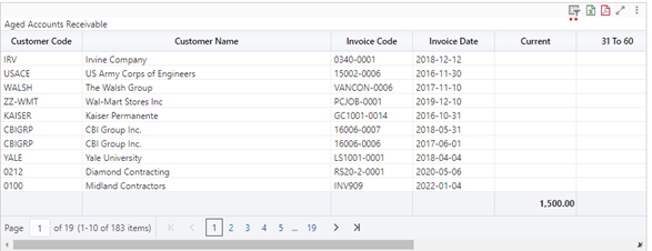
Using the Query by Example method is one of the faster ways to filter data in a table visualization. However, this is not possible in other visualizations, and are not automatically saved (although they can be saved when the BI report is saved). Therefore, this is more of a temporary measure for filtering data. An example is shown below.

Page Filters and Substitution Variables Without the Use of Joins

Page filters and substitution variables are more flexible and dynamic ways to filter data without having to do anything in Catalog Builder. Both page filters and substitution variables are created through the Dashboard or Query drop-down menu on the top left of Dashboard/Query Builder.

While page filters require you to select a field to use as the list of values (LOV), substitution variables allow you to type in a value to apply as a filter.

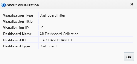
Each page filter or substitution variable has a Visualization ID. This ID can be used to filter data in visualizations.

In the visualization settings, a filter can be applied that refers to the Visualization ID of the page filter or substitution variable, like so:

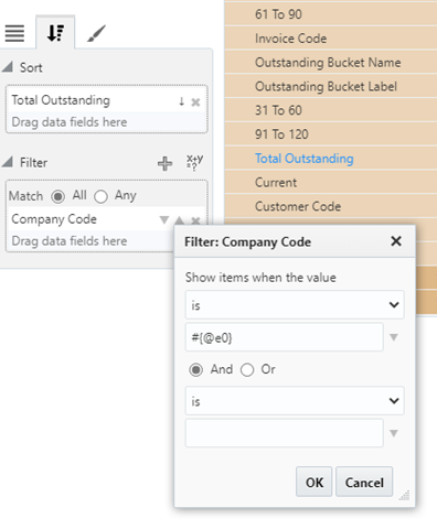
In the above example, the page filter that uses GL Companies as the LOV, is being used to filter the Company Code field in a visualization displaying AR information.

Page Filters with the Use of Joins

It is often convenient to link page filters to visualizations through the use of joins, but this is less efficient than avoiding joins (see previous section). However, it can be convenient to implement a page filter this way.

Select the same field from the page filter and insert it into every visualization that you want to link to the page filter. For example, a page filter that filters the company code from GL Companies will take effect on any visualization that includes GL Companies as part of the selected folders/fields.

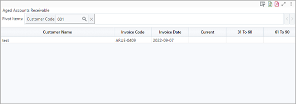
Table Pivot Filters

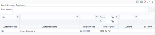
The least efficient way to filter data in a query/dashboard is to use the pivot filters in the table visualization. Dragging a column into the pivot bar (or header bar if the pivot bar is not visible). The process of selecting a value from the pivot filter can be slow as it works to generate the list of values.

Minimizing Joins

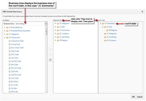
Often, BI visualizations are slow because too many folders are being used (too many joins). In addition, the join tree may be set up to include too many levels. In the example below, the SD Regions folder is three levels deep in the join tree. In this case, selecting fields from the top (JC Summaries) and bottom (SD Summaries) of the join tree is demanding on the server.

Checking the Join Tree icon in the field selector menu allows you to visualize the join tree.

Find ways to select the folders in different orders to avoid making the join tree too large or complex. Sometimes there is low priority information on a visualization that can be removed in order to make the join tree smaller. Alternatively, the visualization can be split into two: the main visualization and a drill-down visualization. More information on setting up drill-downs is in the Dashboard Builder reference guide.

Building Better Joins

When folder joins are necessary, there are some ways to optimize their performance in the Folder Joins screen in Catalog Builder:

• Always use Oraseq fields for joins if they are available. For example, always use Project Oraseq instead of a combination of Project Code and Company Code.

• When creating joins for a new folder in a custom data source, you can use the Import Default Joins functionality to import joins for your new folder from the Default Data Source. This way the user won’t need to guess which fields to use in the joins.

• Avoid using calculated fields for joins.

• Avoid using user extension (UE) fields for joins.

Calculated Fields

Calculated fields can be done in either Query/Dashboard Builder or Catalog Builder. Generally, the more complex a calculated field, the more it makes use of other fields from various folders, the more it will slow down the BI report. Here are some tips to keep in mind when creating calculated fields:

• Minimize the number of fields in the calculation formula.

• If using a SWITCH statement, minimize the number of scenarios that are included.

• Avoid creating a calculated field in Catalog Builder unless the calculated field menu in Query/Dashboard builder is inadequate.

• Avoid using SQL window functions (max() over.. etc.) in Catalog Builder calculated fields. These are known to cause performance issues.

Slow Views

Even when all troubleshooting steps and optimization has been done by the user, it is possible for a BI dashboard or query to be slow. If the customer has a filtered dashboard that is only displaying a few hundred records in each visualization and it is still loading too slowly, then it may be an issue with the folder being selected.

Some folders are more optimized for load speed than others. While CMiC strives to provide the best options in the curated CMiC Default Data Source (Catalog), there may be another database table or view that provides similar information with a faster load speed. If not, you may have to work with a developer to develop a more efficient database view, either through a billable work order or a third-party developer.

Another recommendation is to avoid using views with the # symbol in the name, which you can check in Catalog Builder. These are referred to as fat views and are not ideal for reporting as they are designed to be queried with many columns and few rows. If the fat view is the only view available, it is important to limit the number of rows by using filters.